Simplified Models of the Dolphin Echolocation
Emission System
[Note: This is a draft of an article I started back in 2002. All rights reserved by James L. Aroyan ©
2002. This material may not be
published or distributed without the consent of the author. Educational use is, however,
encouraged. Please provide feedback if
possible.]
Introduction
Can simple acoustic models produce signals having most of the observed characteristics of the echolocation clicks emitted by dolphins? Perhaps surprisingly, the answer is yes.
A simple model corresponding to the acoustic behavior of the dolphin forehead is presented below as both a research and a didactic tool. Movies of simulated sound propagation are used to illustrate the behavior of the individual and combined model components. Only three model components are assumed here: 1) a source mechanism of broadband pulses; 2) one or more damped resonators; and 3) a projector of the signal produced by the first two components. Simple models should be considered qualitative in comparison to more sophisticated modeling techniques. Nevertheless, they serve many purposes including clarification of the mechanisms underlying dolphin biosonar and as a means for exploring how biological tissues interact from an acoustical standpoint. The goal of the current modeling is to illustrate that forehead anatomical variations between odontocete species suggest model parameter (with resulting signal) shifts that correlate with reported differences in signals. A further goal is to find physical explanations for some poorly understood echolocation signal features including:
· The rapid rise and ‘ringing’ decay of the pressure waveforms that are characteristic of the echolocation signals of several odontocete species.
· The observed differences in the number of pressure oscillations within the overall signal envelope for several species.
· Correlations between signal source level and modal frequency composition observed in the bottlenose dolphin, the white whale, and the false killer whale.
· A precursor (or “forerunner”) signal feature.
· Delayed and attenuated signal reverberation features.
· Aspects of the far field distributions of odontocete echolocation signals.
Experimental versions of several simplified models could be built. Such models could serve as ideal laboratory demonstrations for intermediate bioacoustics courses.
It is worth emphasizing that the connections discussed here between dolphin anatomy, echolocation signal analysis, and acoustic models are not new. Many of the references cited in this paper contain far more advanced discussions of dolphin anatomy, echolocation signal analysis, and dolphin bioacoustic modeling. To researchers knowledgeable in both acoustics and biology, most of the material covered here may seem obvious. However, to the best of my knowledge, no one has to date combined these areas in an introductory fashion that accurately communicates the most basic connections. In addition, even the so-called “experts” in the field (some of whom have no understanding of acoustics) do not appear to have appreciated the extent to which simple models can explain the observed characteristics of dolphin echolocation signals.
To make the current topic accessible to the widest possible audience, this paper begins with an overview of the relevant anatomy and a brief description of dolphin echolocation signals.
Overview of Dolphin Forehead Anatomy
This section describes some of the tissues in the dolphin forehead that are thought to play important roles in sound production and emission. For more detailed descriptions of dolphin head and nose anatomy the reader may wish to consult Lawrence and Schevill (1956), Schenkkan (1973), Mead (1975), Green et al. (1980), Heyning (1989), or Cranford et al. (1996).
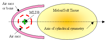
Figure
1 diagrams selected tissues in a parasagittal slice in a plane lying slightly
to the right of the midline of the common dolphin forehead. This diagram includes the skull and jaw bone
(gray hatched), the nasal air sacs (red), the right MLDB complex (including anterior and posterior bursae),
the nasal plug (np), the epiglottic spout (es) of the larynx (blue), and the
melon tissues (yellow gradient). Figure
1 does not illustrate tissues surrounding
the labeled soft tissues and bones, and does not show all air sacs of the upper
nasal passageway.
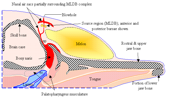
Figure
1. Diagram of selected dolphin head tissues. [Adapted from Aroyan
1990.]
Among other characteristics, all cetacean skulls
exhibit an evolutionary migration of the naris backwards from the tip of the
snout (the typical location in most mammals) to tilt dorsally toward the vertex
of the skull. The cranial vault is
foreshortened and concave, and the maxillary/premaxillary region
elongated. Figure 2 is a photograph of
a common dolphin skull (without the lower jaw). In the common dolphin, the upper naris and the premaxillary
shelves combine to form a roughly semi-parabolic depression of the upper skull
surface. The common dolphin skull also
exhibits a slight displacement of the midline suture to the left, indicating a
directional asymmetry that may mirror related soft tissue asymmetries (the
degree of skull and soft-tissue asymmetry varies considerably among different
odontocetes).
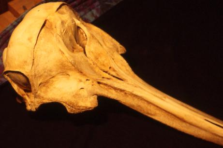
Figure 2. Photograph of common dolphin skull (without lower jaw). The left and right narial passageways through the skull and the supranarial depression are evident.
Figure 3. Diagram of dolphin skull and nasal air sacs. PS – premaxillary sacs (yellow); VS – vestibular sacs (pink); NS – nasofrontal (or tubular) sacs (green); BH – blowhole. Also colored are the spiracular cavity (blue); the skull and upper jaw (light blue); and the lower jaw (light purple). [Adapted from Au 2000; originally adapted from Purves and Pilleri 1983.]
Above the bony naris sit a number of air sacs that
form part of the nasal complex leading up to the blowhole. To better illustrate the 3D structure of the
dolphin’s nasal air sacs, Figure 3 diagrams the air sacs in the inflated
condition associated with the sound production cycle (see below).
Note that the MLDB complexes are located along the dorsal-lateral margins
of the spiracular cavity (colored blue in Figure 3), just below the
floor of the vestibular sacs. The nasofrontal
sacs wrap around the spiracular cavity on either side, and the premaxillary
sacs cover the premaxillary shelves of the skull. The detailed geometry of the nasal sacs varies between species. In the harbor porpoise, for example, the
vestibular sacs have prominent connective tissue ridges along their floors, and
the relative size of these sacs is larger than in most delphinids (Amundin and
Cranford 1980). The commerson’s dolphin
(Cephalorhynchus commersonii) and particularly
the franciscana (Pontoporia blainvillei)
also exhibit relatively large vestibular sacs.
Dolphins and perhaps all odontocetes are capable of creating substantial air pressure (roughly 0.5-1.0 atmosphere above ambient) within their bony naris (Ridgway et al. 1980; Ridgway and Carder 1988), compressed by the large muscles that pull the larynx up toward the narial cavity of the skull. This pressure may be regulated at the top of the narial cavity by the muscular nasal plugs. Several studies (Norris et al. 1971; Dormer 1979; Ridgway et al. 1980; Ridgway and Carder 1988) describe a phonation cycle in which air is pressurized within the bony naris and passed upward into the nasal sac system during production of echolocation clicks and whistles. Air need not be expelled from the blowhole during this cycle – instead, it collects in the distensible vestibular sacs during sound production and is returned to the naris afterward to repeat the cycle.
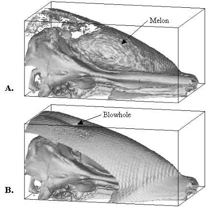
Figure 4.
Visualizations of common dolphin CT data in forehead region. (A) Visualization of skull and outer melon
isosurfaces (portions of the skin surface and nasal sacs are also
visible). (B) Visualization of skull
and skin isosurfaces. [Reproduced from
Aroyan 1996.]
The fatty melon tissues of the dolphin forehead are shown in Figure 1 as a yellow gradient-filled region. These tissues actually consist of a layered topology of lipids that are chemically distinct from blubber and other body fats.[1] The melon rests on a concave pad of connective tissue and musculature above the bony rostrum of the skull. To better illustrate the 3D geometry of the melon tissue within the forehead of the common dolphin, Figure 4 reproduces two CT data visualizations of the skull, melon, and skin isosurfaces from Aroyan (1996).
Velocity measurements over the melon of a bottlenose by Norris and Harvey (1974) revealed a low-velocity core surrounded by higher-velocities that grade into the surrounding muscle and connective tissues. Similar melon structures in other dolphins and porpoises are supported by a growing list of species’ CT and/or MRI scans (Cranford et al. 1996). Wood (1964) was the first of many researchers to suggest that the melon might focus and channel sound generated within the forehead tissues and acoustically couple it to seawater. Computer simulation studies (Aroyan 1990, 1996, 2000; Aroyan et al. 1992) have verified that all of these acoustic behaviors do indeed occur in common dolphin tissue models based on the melon velocity distributions measured by Norris and Harvey (1974).
Some Characteristics of Delphinid Echolocation Signals
Continuing our introduction, we now briefly describe the echolocation signals of dolphins and some other odontocetes. For more detailed information and further references on the characteristics of dolphin echolocation signals, readers are encouraged to consult Au (1993) and Au (2000).
The echolocation signals of odontocete cetaceans have many common features as well as characteristics that differ between species. It is thought that all odontocetes produce short duration (50-400 usec), intense (SL=150-227 dB re 1 uP), and high frequency (12-140 kHz peak frequency) acoustic pulses. The specific ranges within which particular species’ signal parameters fall have been contrasted by many researchers – significant differences do exist in peak frequency, spectral composition, source level, duration, and envelope shape. Some species emit signals having relatively fixed characteristics, making stereotypical descriptions seem appropriate. However, other species appear capable of varying their signal characteristics, and individual animals have been observed to exercise considerable control over their emitted signals. Hence, some flexibility is called for in attempts to categorize species by signal type (or vice versa). It should also be kept in mind that most of the available data on odontocete echolocation signals has been obtained from only a small handful of species.
As an example of the echolocation signals of one delphinid, Figure 5 illustrates a click train emitted by an Atlantic bottlenose dolphin performing a target detection task. The frequency spectrum versus time is plotted on the left and the individual click waveforms are displayed on the right. Peak frequencies for most of the pulses in this click train fall roughly in the 110-120 kHz range, although other components are also visible. The broadband character of these pulses is reflected in –3 dB bandwidths of roughly 60-80 kHz. On average, these signals last only 50-60 ms, a surprisingly short duration considering their biological origin. At a velocity of 1500 m/s in seawater, sound travels 7.5 cm in 50 ms.
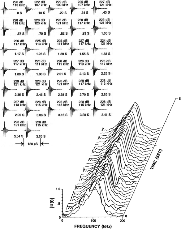
Figure 5.
Signals and spectra of a typical sonar click train emitted by a
bottlenose dolphin (Tursiops truncatus) performing a target detection
task in Kaneohe Bay. The individual
click waveforms are displayed in the upper diagram (with peak-to-peak SL re 1mPa,
peak frequency, and time of click occurrence relative to first click) and the
corresponding frequency spectra vs time of occurrence are plotted in the lower diagram. [Reproduced from Au 1993.]
Examples of sonar signals emitted by a harbor porpoise (Phocoena phocoena) and by a Commerson’s dolphin (Cephalorhynchus commersonii) are provided in Figure 6. Figures 7 & 8 illustrate variations in signals recorded from a bottlenose dolphin (Tursiops truncatus), a beluga or white whale (Delphinapterus leucas), and from a false killer whale (Pseudorca crassidens). These examples fall into two broad categories. The first category consists of higher frequency, narrow bandwidth, and low intensity signals emitted by smaller porpoises and dolphins that do not whistle, exemplified by the signals in Figure 6. The second consists of generally lower frequency, broader bandwidth, and higher intensity signals emitted by larger delphinids and other toothed whales that are capable of whistling (Au 2000), exemplified by the signals in Figures 7 & 8. These categories are not rigid, however, as there is at least one whistling species that also emits high frequency, narrow band, and relatively low intensity signals. Of course, one expects small animals to eat smaller prey, and higher frequency signals enable detection of smaller prey.
From an acoustics standpoint, perhaps the most important thing to note in Figures 5-8 is that all of the signals illustrated appear to be pulses of varied bandwidths that have been filtered by damped resonators. We shall discuss the structures in the dolphin forehead that potentially generate such pulses and cause resonant filtering in the modeling sections of this paper. The acoustical interactions of these structures may indeed provide simple explanations for the different categories of echolocation signals noted above.
The echolocation signal of the Commerson’s dolphin in Figure 6B clearly contains delayed and attenuated signal reverberation features. The delayed signal features in this case create a rippling of the signal spectrum that splits the main spectral peak into three sub-peaks. Careful inspection of Figure 6A also suggests the presence of reverberation features in the signal of the harbor porpoise. The configurations of the soft tissue and air sacs within the left and right nasal passageways of these animals may provide a simple explanation for these reverberation features.
The variability of odontocete echolocation signals is exemplified by Figures 7 & 8 – clearly some animals are able to vary the characteristics of their emitted signals through a wide range.[2] For example, the two signals produced by a bottlenose dolphin in Figure 7 have quite different peak frequencies, bandwidths, and intensities. Nevertheless, some highly significant correlations are present in Figures 5, 7, & 8. It is clear that the spectra in Figures 7 & 8 exhibit bimodal frequency distributions, as do several of the pulses in the click train of Figure 5. Bottlenose dolphin clicks often have peak frequencies in either the 50-60 kHz or the 110-120 kHz ranges. A remarkable series of P. crassidens signals transitioning between a lower frequency mode (~40 kHz) and a higher frequency mode (~110 kHz) is shown in Figure 8B. These variations in modal frequency composition are correlated with signal source level. Au (2000) suggests that “the response of the sound generator may be determined by the intensity of the driving force that eventually causes an echolocation click to be produced.” In musical acoustics, it is common for lip reed sources controlled by air pressure and muscular tension to shift in fundamental frequency and spectral composition as they are driven harder. It would not be surprising if the dolphin’s click generation mechanism were similarly affected by these factors.
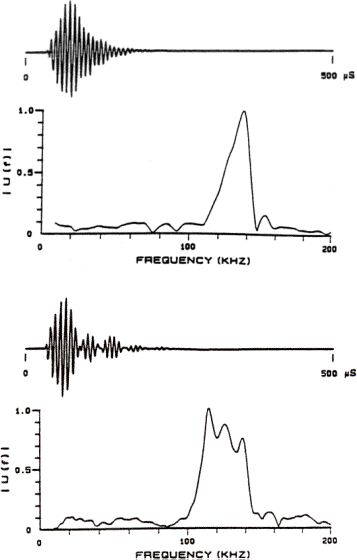

Figure 6. (A) Example of an echolocation signal from
the harbor porpoise (Phocoena phocoena). (B) Example of an echolocation signal from
the Commerson’s dolphin (Cephalorhynchus commersonii). The spectra are plotted below the waveforms. [Signal data from Kamminga and Wiersma
1981. Figure reproduced from Au 2000.]
Note that if the dolphin’s click generator is capable of producing impulses of progressively higher frequency as the driving air pressure and muscular tension is increased, and if this source is located in soft tissues of the nasal passageways that are partially surrounded by air sacs, then the modal characteristics of the spectra in Figures 7 & 8 may simply result from a variable source being filtered by the resonances of a soft tissue resonator (plus a projective filter element). This seems especially apparent in the examples of Figure 8, where it is easy to imagine a relatively fixed bimodal resonator spectrum being driven by a click source that increases its peak frequency with amplitude. Similarly, the narrow bandwidth and reverberant signals of the harbor porpoise and Commerson’s dolphin in Figure 6 may result from more completely air-bounded soft tissue (left and right) cavities that have a higher frequency resonance spectrum (plus a projective filter element). The remainder of this paper explores the implications of such a three-component model of the dolphin echolocation emission system.
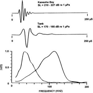
Figure 7. Examples of echolocation signals used by Tursiops truncatus in Kaneohe Bay and in a tank. The spectra are plotted below the pressure waveforms. The dashed curve in the bottom plot is the spectrum of the signal measured in the tank. [Reproduced from Au 2000.]
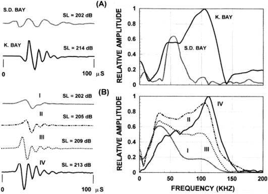
Figure 8. (A)
Example of Delphinapterus leucas echolocation signals in San
Diego Bay and Kaneohe Bay (Au et al. 1985).
(B) Examples of Pseudorca crassidens echolocation signals. The waveforms are shown on the left and the
corresponding spectra on the right. SL
is the averaged peak-to-peak source level in dB re. 1mPa (Au et al. 1995). [Reproduced from Au 2000.]
Simplified Acoustic Model of the Dolphin Forehead
We now consider a simplified acoustical model of the delphinid forehead. This model was proposed in 1996 (Aroyan 1996) but unfortunately was not understood by biological researchers. The model combines three components: 1) a source mechanism of broadband pulses; 2) a damped resonator; and 3) a projector of the signal produced by the first two components.
The source of acoustic pulses is here assumed to correspond to the right MLDB tissue complex (represented by green arrows in Figure 1). The MLDB complexes are located along the dorsal-lateral margins of the spiracular cavity (colored blue in Figure 3), just beneath the floor of the vestibular sacs. The physical mechanism responsible for producing broadband pulses is thought to be pneumatically driven soft tissue oscillations (Cranford et al. 1996; Dubrovsky and Giro 2002). The supranarial depression of the skull and nasal air sacs that partially surround the MLDB soft tissues are assumed to effectively create a damped resonator, causing a resonant filtering of the source spectrum (Aroyan 1996). Finally, a projector of the signal produced by the source and resonator is considered to result from the forward-reflecting portions of the skull and nasal air sacs in combination with the refractive forehead soft tissues (including the melon).
For the purposes of model construction, simplified acoustic versions of the forehead tissues labeled in Figure 1 can be obtained by imagining an axis drawn from the MLDB through the melon core. Figure 9 illustrates a cylindrically symmetric acoustic representation of these tissues. The air sacs partially enclosing the MLDB source region have been simplified to a single spherical sac having gaps through which some of the incident broadband pulse energy escapes. The projector tissues are represented in Figure 9 as including a parabolic air sacs (or bone) reflector and a refractive soft tissue lens.
Figure
9. Simplified cylindrically
symmetric version of model of dolphin forehead tissues.
In the current discussion, it is not critical that the interfaces creating resonances (such as air sacs partially enclosing the source region) be entirely separate from the interfaces contributing to forward reflection. These components are sketched here as being separate in order to clarify the operating mechanisms. Also, it is not crucial whether the shape of the reflector is exactly parabolic (the supranarial depression of the skull, for example, seen in Figure 2, appears approximately semi-parabolic). Finally, although the projector tissues are shown in Figure 9 as consisting of both reflective air sacs (or bone) and refractive forehead soft tissues, it is not crucial to the current argument that there be separate parts to this projective component. For example, the melon could be eliminated from a still-further simplified model, as sketched in Figure 10.
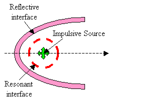
Figure 10. Further simplified sketch of emission model components.
In the following sections, we briefly discuss each of the three assumed components, using movies of simulated wave propagation to illustrate their behavior.
1) Broadband Click Source Component
The anatomical location of the tissues responsible for generating echolocation clicks has in the past been a subject of controversy. Some authors have argued that, as with terrestrial mammals, dolphins produce sounds in their larynx. Nevertheless, almost all experimental studies with live dolphins have implicated the region of the nasal passageways as the origin of echolocation pulses in dolphins. These include cineradiographic studies (Norris et al. 1971, and Dormer 1974, 1979), pulsed ultrasonic imaging (Mackay 1980), ultrasonic Doppler-shift motion detection (Mackay and Liaw 1981), pressure sensing and electromyographic studies (Ridgway et al. 1980), and direct palpation during sound production (Amundin 1990). Two recent studies have narrowed the location of the source tissues down to the upper nasal passages, just beneath the floor of the vestibular sacs (see Figure 3). Aroyan (1996) simulated acoustic propagation within 3D forehead tissue models of D. delphis using techniques analogous to those applied in seismology to locate the epicenters of earthquakes. A close clustering of focal centers for forward-directed beams was found that best supports the right MLDB complex as the source of echolocation clicks in this dolphin (Aroyan et al. 2000). In addition, Cranford et al. (2000) observed motions of the MLDB complexes correlated with click production in T. truncatus. Although Cranford et al. (2000) did not rigorously exclude other tissues as potential sources, their observations suggest that both left and right MLDB complexes are capable of generating echolocation clicks.
Closely related to source location issues are questions concerning the exact physical mechanism by which clicks are produced. Many of the studies referenced above have suggested source mechanisms, but few of these suggestions are based on solid acoustical arguments. Perhaps the most convincing work to date in this area is summarized in Dubrovsky and Giro (2002). Physical and mathematical models of a source mechanism are described (Giro 1987; Dubrovsky and Giro 2002) in which brief (50-80 msec), high frequency (fpeak around 100kHz), and broadband (up to 80 kHz –3dB widths) pulses result from surface accelerations during pneumatically driven oscillations. For the purpose of modeling the dolphin emission system, this suggests that a small source of broadband pulses should be considered to be the first component of the system.
At this point in our discussion, let us momentarily turn our attention to the visualization of sound propagation when exploring various models. For visualization purposes, we will use finite-difference time-domain (FDTD) wave propagation programs in which symmetry about the z-axis is assumed. This simplifying assumption does not overly restrict our ability to explore basic models. The geometry of the simulation grid is diagrammed in Figure 11. Z-axis symmetry allows us to reduce the simulation grid to a half-plane that includes the z-axis. If absorbing boundary conditions are added along all boundaries other than the symmetry axis, then only a small portion of the half-plane containing the model needs to be simulated. This approach allows us to compute sound fields rapidly and to illustrate the full 3D solutions in time with 2D grid movies. In all movies presented below, the simulation grids represent half of a 2D slice through the center of our 3D (axisymmetric) models. Height above the plane in these movies represents the acoustic pressure of the propagating wave solutions.
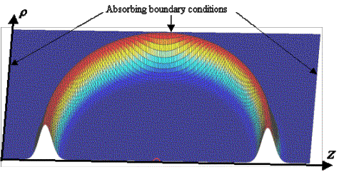
Figure 11. Simulation grid geometry: rotational symmetry about the z-axis is assumed, and variable r represents distance from the z-axis. Gaussian pulse propagation snapshot.
(If movie does not
start on a Windows PC, download file “Movie1.wmv” to your computer, then
run it with Windows Media Player or another video app that accepts “wmv”
format. Apologies for the
Mac-unfriendly format – contact me via email for the individual movie frame
images.)
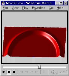
Figure 12. Movie of Gaussian pulse emission by the
source (click on figure to start).
As an example, the waveform in Figure 11 is a snapshot of a Gaussian pulse (Figure 14A) that was emitted from a small source (the small semi-circle on the z-axis). The full 3D solution is just this waveform rotated about the z-axis – i.e., a spherical wave spreading away from the source point. A movie of the Gaussian pulse emission by the source and its absorption by the boundary conditions is provided in Figure 12.
In all simulations in this report, we will use fixed length and time scales. These scales are established by the dimensions of our model on the grid and by the relevant wave velocity. Here we choose 152 grid increments to correspond to 5.00 cm, making 1 grid increment equivalent to Dh @ 0.329 mm. Waves traveling at the nominal simulation velocity cover k @0.612 grid increments per time step. Assuming this nominal velocity corresponds to a speed of sound in seawater of c @ 1.53106 mm/s, then one simulation time step corresponds to Dt = k (Dh / c) @ 0.134 ms. Given these values of Dh and Dt, the above Gaussian pulse would then have a –3dB bandwidth of 148 kHz (74 kHz in positive frequency) and a duration of about 4.2 ms (FWHM time-record of pressure). The dimensions of the simulation grid in Figure 12 are then 6.58 cm by 13.16 cm.
Now let us continue with our discussion of the source mechanism. Certain features of the frequency spectrum of a source are directly attributable to its physical characteristics. For example, if the surface area of the source is small, the low-frequency end of the spectrum is necessarily reduced by the low emission efficiency of small sources at large wavelengths. Also, at the high-frequency end, the spectral energy must be limited by the finite acceleration of real surfaces – biological tissues cannot undergo infinite accelerations. Furthermore, one would expect both the peak frequency and the maximum emitted pulse amplitude to increase with increasing surface accelerations. In the case of air pressure driving tissue oscillations, it makes physical sense to suggest that both the peak frequency fpeak and the maximum amplitude Apeak may be controlled by increasing or decreasing the driving pressure. All of these factors support the assumption of a broadband source with both fpeak and Apeak dependent on driving pressure (among other variables). Figure 13 represents a qualitative plot of such a source spectrum.
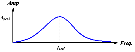
Figure 13. Qualitative plot of assumed broadband source spectrum.
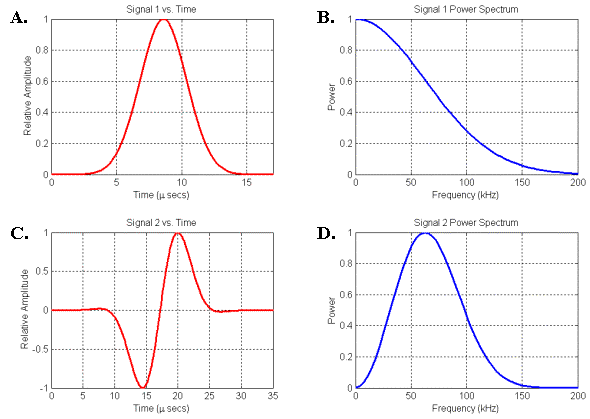
Figure
14. Two signals and their associated power spectra. (A) Gaussian signal. (B) Spectrum of signal in A. (C) Gaussian-windowed sinusoid signal. (D) Spectrum of signal in C.
Figure 14 illustrates two types of pressure pulses and their corresponding frequency power spectra. Figures 14A-B plot the signal and spectrum of the Gaussian pulse propagated in the movie of Figure 12. Figures 14C-D plot the signal and spectrum of a Gaussian-windowed sinusoid pulse. The low-frequency end of the spectrum in Figure 14D agrees more closely with the spectral characteristics plotted qualitatively in Figure 13 than does the low-frequency end of Figure 14B. [Figure 14D should also be compared with Figure 6 in Dubrovsky and Giro (2002)]. In other words, for physical reasons we do not expect a small soft-tissue source to emit pure Gaussian-type signals – a Gaussian-windowed sinusoid represents a closer match to the expected spectral characteristics. Nevertheless, we will use Gaussian source signals in some of the following simulation movies because they create propagation patterns that are often simpler to visually interpret.
The exact structure of the waveforms generated by pneumatically-driven soft tissue motions depends on several variables, of course. The elastic properties of the tissues, the driving air pressure and air flow characteristics, and tissue size and geometry might all be expected to influence the waveform structure. From the standpoint of model construction, however, it is not critical that we know the exact structure of the input waveform. Indeed, it may be possible to infer the input waveform of the remarkable progression of signals shown in Figure 8B, for example, by postulating that a fixed resonator spectrum is being driven by an input pulse of sequentially increasing peak frequency, intensity, and bandwidth. The freedom that models provide to explore the consequences of basic assumptions is one of their principle advantages.
2) Damped Resonator Component
A resonant component is suggested by the many reflective structures that partially surround the soft (source) tissues within the dolphin’s nasal passages – acoustically these structures should create resonant interactions in addition to forward reflections. It is also suggested by the decay-like characteristics of odontocete echolocation signals – these signals are strongly reminiscent of the responses of resonators (one or more – with resonant spectra dependent on species) to broadband pulse inputs. In the discussion below, we first visualize the behavior of a resonator driven by an impulsive input. Next we consider a little theory for a simple spherical (partially air-bounded) resonator in order to obtain a general idea of its expected filtering effects. Finally we illustrate some examples of dolphin-like signals generated by simple resonator models driven by broadband sources of the type discussed in the previous section.
What happens to an outward propagating pulse if we partially surround the source region with air spaces? This is not hard to simulate, so let’s try it. Figure 15 illustrates a movie of the same outward propagating pulse as in Figure 12, but this time surrounded by a few equally spaced “air sac” points on the (green) circle surrounding the source. Instead of the single outward propagating pulse that we saw in Figure 12, Figure 15 illustrates a decaying series of oscillations propagating away from the resonator. Figure 16 is a plot of these oscillations recorded at the center of the simulation grid.
(If movie does not start on a Windows PC, download
file “Movie2.wmv” to your computer, then run it with Windows Media Player
or another video app that accepts “wmv” format. Apologies for the Mac-unfriendly format – contact me via
email for the individual movie frame images.)
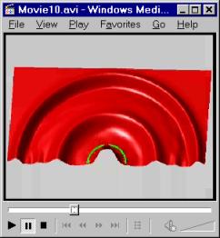
Figure 15.
Movie of Gaussian pulse emission by a partially air-bounded source
(click on figure to start). The resonator diameter is 2.5 mm (indicated
by green circle).
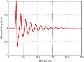
Figure 16. Plot of the signal recorded at the center of the grid in Figure 15 movie.
What causes these oscillations? The air-filled sacs within soft tissue act like very good mirrors reflecting and/or scattering almost all sound incident upon them. Depending on the soft-tissue sound speed distribution and the geometry of the air sacs and source, resonances (or nulls) are created by reinforcement (or interference) of the reflections within any such enclosure. The resonator model is simply responding with its characteristic spectrum to the Gaussian pulse that was input at its center. As we shall see below, for some simple enclosure and source geometries, the expected resonance spectra can be calculated.[3] In cases involving more complicated geometries such as the dolphin nasal air sac system, time-domain simulation is an excellent way to determine the characteristic spectrum of the nasal air sac resonator.
As a highly simplified theoretical example, consider the case of a completely air-bounded spherical soft-tissue enclosure. A completely air-bounded enclosure would approximate an undamped resonator. Taking the speed of sound within the soft tissue volume to be c=1500m/s, and the radius to be r=1.25cm, the first two sets of radial modes would be:
Monopole
(0th order) Radial Modes:
The frequency of the nth monopole radial mode is just the nth harmonic of f0,1=60kHz:
f0,n = n f0,1 = n (c/2r) = n (60 kHz).
Dipole (1st order)
Radial Modes:
The dipole radial mode does not contribute harmonics. Instead, the first three resonant frequencies are:
f1,1 = 85.8 kHz, f1,2 = 148 kHz, f1,3 = 208 kHz.
A centered monopole source, however, would be expected to couple primarily into the monopole radial modes, and the resonant structure of such an enclosed source should be predominantly harmonic. Although the symmetry properties of the click source mechanism in dolphins are not yet known, we can simply assume a monopole source for our present modeling purposes. Figure 17 sketches the monopole mode spectrum for an air-bounded spherical soft-tissue enclosure.
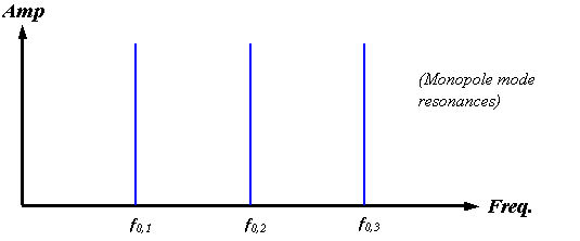
Figure 17.
Sketch of the lowest order radial mode harmonics of a completely air-bounded
spherical enclosure. A harmonic series
of delta functions occurs in this case.
Of course, the nasal air sacs pictured in Figure 3 do not entirely enclose the soft tissue source region (here assumed to be the right MLDB complex). A partially air-bounded enclosure creates decaying oscillations as sound “leaks out” of the enclosure. Instead of the infinitely high and narrow delta functions sketched in Figure 17, the cavity resonances broaden and weaken by amounts that depend on the fraction of the surface enclosed by air, its geometry, and the resonant frequencies. Figure 18 qualitatively indicates how this might modify the spectrum of Figure 17.
Note that we are discussing the response or filter spectrum of the resonator component here, and not the combined system. We have not yet considered the filtering effect of projecting or focusing the signal into a beam. The filtering created by the final (projector) component will be discussed in the next section. Even if certain tissues within the dolphin forehead contribute to more than one of the three model component behaviors discussed here, it is still possible to model each stage in the emission process separately – that is, as having a well-defined spectral filtering effect. As we shall see below, linear systems theory tells us how to combine the component filters into a complete model (see also Appendix 1).
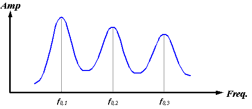
Figure 18. Sketch of a possible spectrum of a partially air-bounded spherical enclosure.
To conclude this section, let’s consider some specific examples of dolphin-like signals generated by simple resonator models driven by broadband source pulses. Figure 19 illustrates three different input (or driving) and output (or response) signals generated by another simple resonator model. This model consists of a circle of points surrounding the source with a velocity lower than the surrounding medium. Because of the axial symmetry of the simulation, this model corresponds physically to a thin spherical shell of lowered (perturbed) velocity. The value of the velocity perturbation in this model can be adjusted to create varying resonance strengths (or Q-values) – note that the resonance peak frequencies also vary with the velocity perturbation. Because of the spherical symmetry of this model, there is no directional variation in the emitted signal; hence we may record the resulting signal anywhere outside the resonator model.
The first two response signals of this simple model (Figures 19B, 19D) are similar to the two variations of bottlenose dolphin echolocation clicks shown in Figure 7. The response signal seen in Figure 19F is similar to the harbor porpoise echolocation click shown in Figure 6. The center frequencies, bandwidths, and phases of the input signals (Figures 19A, 19C, 19E) were adjusted to yield responses that approximate the shapes of the recorded echolocation clicks. The center frequencies of signals D and F are only roughly matched to the echolocation clicks shown in Figures 6 & 7 – to get closer matches, one needs to match the modal frequencies of the model to the echolocation click peak frequencies (this can be done by changing the radius of our simple spherical shell resonator model). All three input signals are Gabor functions with the zero-frequency component removed.[4]
It should be emphasized that a wide variety of dolphin-like response signals are obtainable by varying the peak frequency, bandwidth, and phase of the driving signals – this is obvious from a signal processing perspective. In addition, varying of source positioning within the resonator will affect its coupling into the natural modes of the resonator – this is obvious from an acoustical perspective. If all of these factors are allowed to vary along with resonator model geometry, it becomes clear that a very wide range of signals similar to dolphin echolocation clicks can be produced. In principle, though, these variations all result from driving simple resonator models with broadband pulse inputs.
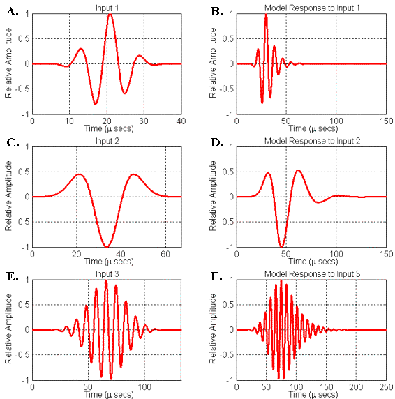
Figure 19. Simulated responses of a simple spherical shell resonator model to signals input at its center. (A) Input signal 1. (B) Resonator response to input 1. (C) Input signal 2. (D) Resonator response to input 2. (E) Input signal 3. (F) Resonator response to input 3.
It is worth mentioning two additional connections between these simple models and observed echolocation click characteristics. First, the longer decay of the signal in Figure 19F was produced using a more resonant model (the velocity perturbation of the spherical shell model was increased in this case). In the case of an air-bounded soft tissue resonator, increasing the amount of air-covered surface around the source greatly increases the strength of the cavity resonances. As mentioned in the anatomy overview, the harbor porpoise, the commerson’s dolphin, and the franciscana are known to have relatively larger air sacs enclosing the nasal soft tissue region. It thus makes sense that their recorded echolocation signals exhibit significantly longer decays.
Second, the left and right sides of the nasal air sacs in some odontocetes may actually create two coupled resonant cavities. If two resonators having similar resonances are placed side by side and one is driven with a broadband pulse, delayed and attenuated reverberations generally occur some time after the beginning of the initial response. The echolocation clicks of the Dall’s porpoise (Phocoenoides dalli), the Commerson’s dolphin (Cephalorhynchus commersonii), and some other odontocetes (Au 1993) exhibit delayed components. Close examination of the harbor porpoise echolocation click and its spectrum shown in Figure 6 indicates that some delayed signal components are present in this species as well. Dudok van Heel (1981), Kamminga and Wiersma (1981), and Wiersma (1982) have all suggested that these delayed low-amplitude signal components are reverberations due to reflections from the skull and/or nasal air sacs. In general support of this idea, the time separation of the signal reverberations for all five animals pictured in Figure 7.20 of Au (1993) appears to scale approximately with their relative size. The exponential amplitude dropoff seen in subsequent reverberations also generally supports a coupled resonator reverberation hypothesis.
Most recordings of dolphin echolocation clicks are measured at some distance in front of the animal that emits the click. This means that these recordings actually include the filtering effect of the beam-forming or focusing produced by the forehead tissues. The next section discusses this final filtering component of the emission system.
3) Reflective and/or Refractive
Projector Component
The signal produced by a nasal click source (and resonator) must pass through the dolphin’s forehead tissues before entering seawater. The forward-reflective properties of the skull and nasal sacs and the refractive properties of the melon and other forehead soft tissues combine to produce additional filtering of the signal. For this reason, a “projective” element is considered to be the third and final component of the dolphin emission model.
Beam-forming lenses or mirrors are essentially spatial filters that are peaked in some focal direction. While descriptions of lens and mirror behavior can be found in any elementary optics textbook, in the discussion below we will add a couple of less well-known properties that are relevant to modeling the dolphin echolocation system.
Let’s begin by considering the behavior of a refractive lens. The shape of the lens, the distribution of refractive index within the lens, and the positioning of the source with respect to the lens are obvious factors that affect refractive focusing by the lens. In addition, for the range of frequencies of interest to dolphin biosonar, the wavelengths are not small in comparison to the dimensions of the refractive forehead soft tissues. Hence diffractive effects also need to be included in an appropriate filter model (in this case, lens filtering depends on both direction and frequency). For common lens shapes and finite wavelengths, diffractive effects generally produce a high-pass frequency filtering in the focal direction.
Similarly, a simple parabolic reflector constitutes a combined directional and frequency filter element. The geometrical acoustics directional pattern for a source at the focus of a true parabola would be a delta function in the focal direction. In the case of a finite aperture/wavelength ratio, however, diffraction modifies this pattern into a high-pass (or high-boost) frequency filter in the focal direction, where the knee of the boost transition frequency depends on the aperture size (and focal distance) of the parabola.
![]()
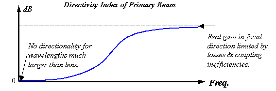
Figure 20.
Qualitative plot of the directivity index of the primary beam versus
frequency for a real projector element.
Figure 20 illustrates what the high-pass filtering might look like for a semi-parabolic reflector and/or lens element (or a model combining both) assuming that the projector creates a primary beam. Figure 20 qualitatively plots the directivity index (DI) of this primary beam versus frequency. Clearly, diffraction must eliminate the peak for wavelengths much larger than the projector. In other words, because waves spread uniformly in all directions in the low-frequency limit, the DI must approach zero as f®0. Furthermore, some acoustic ‘leakage’ and coupling inefficiencies always exist in real systems, and this limits the gain that is possible in the focal direction. Hence directivity indexes for real systems generally level out to yield a finite boost in the high-frequency limit.
Three-dimensional simulations of the focal characteristics of the forehead tissues of the common dolphin do in fact produce directivity indexes that follow this type of curve. Figure 21
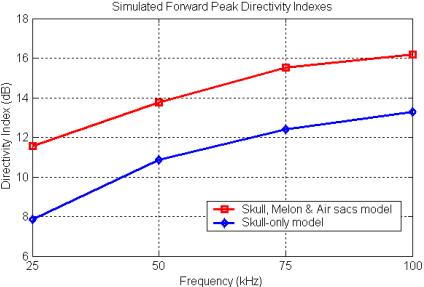
Figure 21. Plot of the simulated directivity index of
the forward peak versus frequency for two different 3D forehead tissue models
of the common dolphin (data from Aroyan 1996).
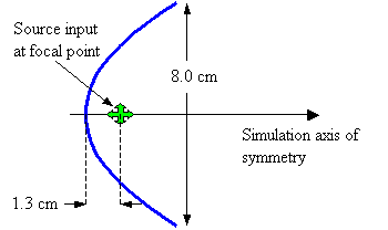
Figure 22. Assumed geometry of parabolic reflector model.
plots out the simulated DI values for the forward peak for two different tissue models from Aroyan (1996). Note that the range of simulated frequencies in this study spanned only a portion of the upper knee of the transition region. The most complete tissue model (the skull, melon & air sacs model) clearly creates a more focused forward beam than the skull-only model. We might also note that by around 100 kHz, the common dolphin is gaining most of the beam-forming benefit of its projector element (as modeled).
Now let’s check out the behavior of some simple projector models. First, let’s consider a parabolic reflector having the dimensions diagrammed in Figure 22. In this model, the reflector is composed of air sacs (discretely modeled pressure release points). The aperture diameter is 8.0 cm (model rotated about the symmetry axis), and the source is placed at the focus of the parabola at a distance of 1.3 cm from the vertex. Although this example may appear trivial, two non-trivial details of potential relevance to dolphin echolocation emission are discussed below.
Figure 23 illustrates a movie of the emitted waveform when a Gaussian pulse (Figure 14A) is input into the focus of the parabolic reflector model diagrammed in Figure 22. The emitted signal was recorded (on an enlarged simulation grid) at a distance of 30 cm to the right of the focal point along the symmetry axis, and is displayed along with its power spectrum in Figure 24. The far field pattern for the emitted waveform forms at around 15 cm from the focus, so the signal in Figure 24A is representative of the emitted far field signal along the primary axis.
Note first that a forerunner (or precursor) signal is seen in both the movie and the signal waveform (Figure 24A). This precursor is simply the portion of the source pulse that did not strike the reflector, and therefore continues to spread (spherically if no other elements are present) from the source point. The ratio of amplitudes of the precursor to the main signal approaches a constant value in the far field that depends on several factors. This precursor is not reflected and hence is not filtered by the reflector element’s transfer function. In our simple reflector model, it therefore cleanly represents the original source pulse. Multiple reflections within the dolphin’s more complicated forehead tissues, however, may mix the precursor and main signal components (especially for longer source pulses).[5]
(If movie does not start on a Windows PC, download
file “Movie3.wmv” to your computer, then run it with Windows Media Player
or another video app that accepts “wmv” format. Apologies for the Mac-unfriendly format – contact me via
email for the individual movie frame images.)
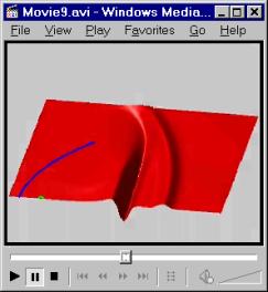
Figure 23. Movie of the waveform emitted by the parabolic reflector model diagrammed in Figure 22 using a Gaussian input (click on figure to start). The reflector location is indicated by the blue curve, and the source (focal) point by a small green semi-circle.
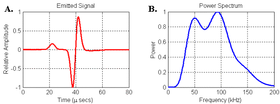
Figure 24.
(A) Waveform and (B) power spectrum of the signal emitted by the
parabolic reflector model. Signal was recorded
at 30 cm along model axis from focal point of parabola.
The second thing to note is that the spectrum of the emitted signal in Figure 24 contains two broad resonances that look similar to the bimodal spectra of some bottlenose dolphin and beluga clicks. In order to understand this result, it is perhaps better to consider the transfer function linking the input and output of the reflector model rather than its response to any one input. Since we know both the input and the output (emitted) waveforms in this model, we can use spectral methods to calculate the filter spectrum of the reflector model itself (see Appendix 1).
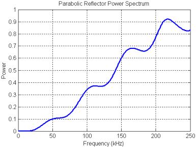
Figure 25. Power spectrum of the filtering created by the parabolic reflector model.
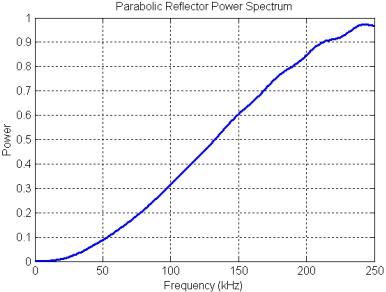
Figure 26. Power spectrum of the parabolic reflector model calculated with the precursor pulse gated out of the received signal.
The power spectrum of the parabolic reflector is plotted in Figure 25. The filtering produced by the parabolic reflector is mainly a treble boost spectrum (qualitatively sketched in Figure 20) with some smaller oscillations superimposed. These oscillations are due primarily to a delayed-signal component (a pure delay spectrum has much stronger peaks and nulls). The mild resonances at around 55, 110, 165, and 220 kHz result from the rippled-spectra of the pulse ‘echo’ reflected off the parabola. This can be demonstrated by gating out the precursor in the received signal (Figure 24A), then computing the reflector transfer function again. The result, shown in Figure 26, retains the treble-boost spectrum of Figure 25 but loses most of the superimposed oscillations. Note that adding a refractive lens in front of this reflector model might lower the frequency of the boost transition, but probably would not affect the resonance features of Figure 25.
The rippled-spectra portion of Figure 25 appears to correlate with the even peaks of an echo spectrum having (roughly) a 30 kHz fundamental, which is somewhat unexpected for this model. Recall that the reflector is modeled as a pressure release surface. Pressure release surfaces invert the phase of reflected waveforms, so one might have expected this reflector to create an inverted and delayed Gaussian pulse following the precursor (ignoring other subtleties) – this does indeed occur very close to the reflector surface (as seen in the movie). A signal consisting of pure delayed and inverted pulses has spectral peaks at the odd (n = 1,3,5…) harmonics of the fundamental delay frequency. The delay is approximately Dt = 2*a/c = ~17 ms, where a = 1.3 cm is the parabola focal distance, and c = 1500 m/s is the assumed sound speed. This yields an expected rippled-spectra fundamental of f = 1/(2*Dt) = 29 kHz. A signal consisting of delayed but non-inverted pulses has spectral peaks at the even (n = 0,2,4…) harmonics of the fundamental delay frequency.
The main part of the emitted pulse in Figure 24A is not merely a phase-inverted copy of the initial pulse, even though it starts out this way. The movie illustrates that a crest following the inverted pulse begins to develop even before it has completely exited the reflector. Some energy can be seen scattering off the end of the reflector, and the scattered wavefronts eventually contribute to the formation of the crest. Decreasing the aperture size of the reflector model increases the magnitude of the resonances and also increases the frequency of the boost transition. The mild resonances in the spectra of parabolic reflectors may be of some importance because they provide a simple way to generate pulses with bimodal spectra similar to the recorded clicks of bottlenose dolphins (and other odontocetes). Driving a parabolic reflector with pulses having spectra peaked near these resonances produces signals very similar to the clicks in Figures 6-8.
Behavior of Combined Elements
Now imagine an acoustical system combining the three elements described above. … To be completed.
Summary of Conclusions
To be completed.
Appendix on Spectral Methods
To be completed.
References:
Amundin M, Cranford T (1990) Forehead anatomy of Phocoena phocoena and Cephalorhynchus commersonii: 3-dimensional computer reconstructions with emphasis on the nasal diverticula. In Thomas JA, Kastelein R (eds), Sensory abilities of cetaceans : Laboratory and field evidence. New York: Plenum, pp. 1-18.
Aroyan JL (1990) Numerical simulation of dolphin echolocation beam formation. M.S. thesis, University of California, Santa Cruz.
Aroyan JL (1996) Three-dimensional numerical simulation of biosonar signal emission and reception in the common dolphin. Ph.D. dissertation, University of California, Santa Cruz.
Aroyan JL, McDonald MA, Webb SC, Hildebrand JA, Clark D, Laitman JT, Reidenberg JS (2000) “Acoustic Models of Sound Production and Propagation.” In: Au WWL, Popper AN, Fay RR (eds), Hearing by Whales and Dolphins. New York: Springer-Verlag, pp. 409-469.
Aroyan JL, Cranford TW, Kent J, Norris KS (1992) Computer modeling of acoustic beam formation in Delphinus delphis. J. Acoust. Soc. Am. 92:2539-2545.
Au WWL (1993) The Sonar of Dolphins. New York: Springer-Verlag.
Au WWL (2000) Echolocation in Dolphins. In: Au WWL, Popper AN, Fay RR (eds), Hearing by Whales and Dolphins. New York: Springer-Verlag, pp. 364-408.
Cranford TW (1992) Functional Morphology of the Odontocete Forehead: Implications for Sound Generation. Ph.D. dissertation, University of California, Santa Cruz.
Cranford TW, Amundin M, Norris KS (1996) Functional morphology and homology in the odontocete nasal complex: implications for sound generation. J. Morph. 228:223-285.
Dubrovsky NA, Giro LP (2002) Modeling of the clicks production mechanism in the dolphin. In Thomas JA, Moss C, and Vater M (eds), Echolocation in Bats and Dolphins. Univ. Chicago Press (in press).
Dudok van Heel (1981) Investigations on cetacean sonar III: A proposal for an ecological classification of Cetacetes in relation to sonar. Aquat. Mamm. 8:65-68.
Fraser FC, Purves PE (1960) Hearing in cetaceans: evolution of the accessory air sacs and the structure and function of the outer and middle ear in recent cetaceans. Bull. British Mus. (Nat. Hist.), 7:1-140.
Giro LR, Dubrovskiy NA (1973) On the origin of low-frequency component of the echoranging pulsed signal of dolphins. In Ref. Dokl. 8-ya Vses. Akust. Konf. (Proceedings of the 8th All-Union Acoustics Conference), Moscow, 1973.
Giro LR, Dubrovskiy NA (1974) The possible role of supracranial air sacs in the formation of echo ranging signals in dolphins. Akust. Zh., 20(5):706-710.
Green RF, Ridgway SH, Evans WE (1980) Functional and descriptive anatomy of the bottlenosed dolphin nasolaryngeal system with special reference to the musculature associated with sound production. In Busnel RG, and Fish JR (eds), Animal Sonar Systems. New York: Plenum, pp. 199-238.
Heyning JH (1989) Comparative facial anatomy of beaked whales (Ziphiidae) and a systematic revision among the families of extant Odontoceti. Contributions in Science, Nat. Hist. Mus. of Los Angeles County, 405:1-64.
Kamminga C, Wiersma H (1981) Investigations on cetacean sonar II: Acoustical similarities and differences in odontocete sonar signals. Aquat. Mamm. 8(2):41-62.
Lawrence B, Schevill WE (1956) The functional anatomy of the delphinid nose. Mus. Comp. Zool. Bull., 114(4):103-151.
Litchfield C, Karol R, Mullen ME, Dilger JP, Luthi B (1979) Physical factors influencing refraction of the echolocative sound beam in Delphinid Cetaceans. Mar. Bio. 52:285-290.
Mead JG (1975) Anatomy of the external nasal passages and facial complex in the Delphinidae (Mammalia: Cetacea). Smithsonian Contr. Zool. 207:1-72.
Moore PWB, Powloski D (1990) Investigation of the control of echolocation pulses in the dolphin (Tursiops truncatus). In Thomas JA, Kastelein R (eds), Sensory abilities of cetaceans : Laboratory and field evidence. New York: Plenum, pp. 305-316.
Morris R (1986) The acoustic faculty of dolphins. In: Bryden MM, Harrison R (eds), Research on Dolphins. New York: Clarendon, pp. 369-399.
Norris KS (1964) Some problems of echolocation in cetaceans. In: Tavolga WN (ed), Marine Bio-acoustics, Vol. 2. New York: Pergamon, pp. 317-336.
Norris KS (1968) The Evolution of Acoustic Mechanisms in Odontocete Cetaceans. In: Drake ET (ed), Evolution and Environment. New Haven: Yale University Press, pp. 297-324.
Norris KS, Evans WE, Turner RN (1966) Echolocation in an Atlantic bottlenose porpoise during discrimination. In Busnel RG (ed), Animal Sonar Systems: Biology and Bionics. Frascati, Italy, pp. 409-437.
Norris KS, Harvey GW (1974) Sound transmission in the porpoise head. J. Acoust. Soc. Am. 56:659.
Oelschlager HA (1986) Comparative morphology and evolution of the otic region in toothed whales (Cetacea: Mammalia). Am. J. Anat. 177:353-368.
Purves PE, Pilleri G (1983) Echolocation in Whales and Dolphins. Academic Press, London.
Popper AN (1980) Sound emission and detection by delphinids. In: Herman LM (ed) Cetacean Behavior: Mechanisms and Functions. New York: John Wiley & Sons, pp. 1-52.
Schenkkan EJ (1973) On the comparative anatomy and function of the nasal tract in odontocetes (Mammalia, Cetacea). Bijdragen tot de Dierkunde 43(1):93-112.
Varanasi U, Feldman HR, Malins DC (1975) Molecular basis for formation of lipid sound lens in echolocating cetaceans. Nature 255:340-343.
Varanasi U, Markey D, Malins DC (1982) Role of isovaleroyl lipids in channeling of sound in the porpoise melon. Chem. Phys. Lipids 31:237-244.
Wiersma H (1982) Investigations on cetacean sonar IV: A comparison of wave shapes of odontocete sonar signals. Aquat. Mamm. 9(2):57-67.